Grasping Gradient Descent using Python

Documenting and sharing everything I learn about Data Science, Machine Learning, R, Python, SQL and more.
Organizational psychologist turned data scientist
Photo by Fineas Anton on Unsplash
Overview
In this post, we'll explore Gradient Descent from the ground up starting conceptually, then using code to build up our intuition brick by brick.
While this post is part of an ongoing series where I document my progress through Data Science from Scratch by Joel Grus, for this post I am drawing on external sources including Aurélien Geron's Hands-On Machine Learning to provide a context for why and when gradient descent is used.
We'll also be using external libraries such as numpy, that are generally avoided in Data Science from Scratch, to help highlight concepts.
While the book introduces gradient descent as a standalone topic, I find it more intuitive to reason about it within the context of a regression problem.
Setup
In any modeling task, there is error, and our objective is minimize the errors so that when we develop models from our training data, we'll have some confidence that the predictions will work in testing and completely new data.
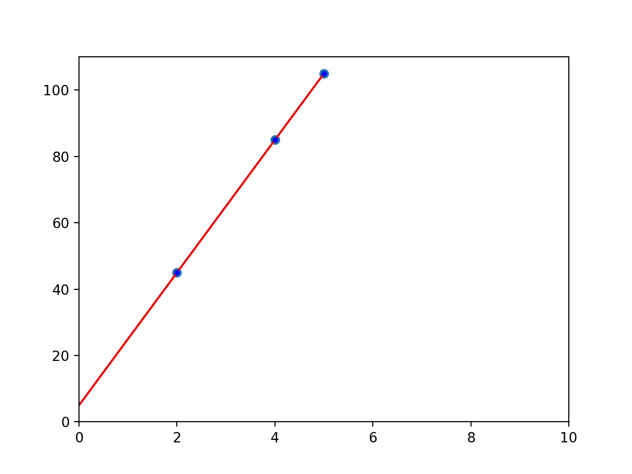
We'll train a linear regression model. Our dataset will only have three data points. To create the model, we'll setting up parameters (slope and intercept) that best "fits" the data (i.e., best-fitting line), for example:
We know the values for both x and y, so we can calculate the slope and intercept directly through the normal equation, which is the analytical approach to finding regression coefficients (slope and intercept):
# Normal Equation

import numpy as np
import matplotlib.pyplot as plt

x = np.array([2, 4, 5])
y = np.array([45, 85, 105])

# computing Normal Equation
x_b = np.c_[np.ones((3, 1)), x]       # add x0 = 1 to each of three instances
theta = np.linalg.inv(x_b.T.dot(x_b)).dot(x_b.T).dot(y)

# array([ 5., 20.])
theta
The key line is np.linalg.inv() which computes the multiplicative inverse of a matrix.
Our slope is 20 and intercept is 5 (i.e., theta).
We could also have used the more familiar "rise over run" ((85 - 45) / (4 - 2)) or (40/2) or 20, but we want to illustrate the normal equation which should come in handy when we go beyond the simplistic three data point example.
We could also use the LinearRegression class from sklearn to call the least squares (np.linalg.lstsq()) function directly:
# Least Squares

from sklearn.linear_model import LinearRegression
import numpy as np

x = np.array([2, 4, 5])
y = np.array([45, 85, 105])

x = x.reshape(-1, 1)              # reshape because sklearn expect 2D array

x_b = np.c_[np.ones((3, 1)), x]   # add x0 = 1 to each of three instances

theta, residuals, rank, s = np.linalg.lstsq(x_b, y, rcond=1e-6)

# array([ 5., 20.])
print("theta:", theta)
This appraoch also yields the slope (20) and intercept (5) directly.
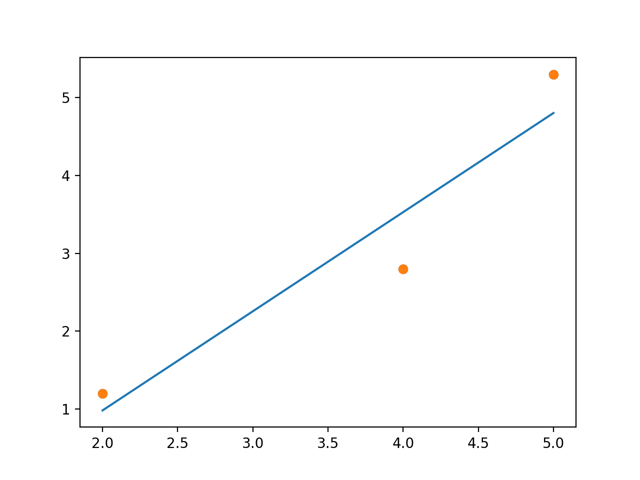
We know the parameters of x and y in our example, but we want to see how learning from data would work. Here's the equation we're working with:
y = 20 * x + 5
And here's what it looks like (intercept = 5, slope = 20)
Gradient Descent
Why?
The normal equation and the least squares approach can handle large training sets efficiently, but when your model has a large number of features or too many training instances to fit into memory, gradient descent is an often used alternative.
Moreover, linear least squares assume the errors have a normal distribution and the relationship in the data is linear (this is where closed-form solutions like the normal equation excel). When the data is non-linear, an iterative solution (gradient descent) can be used.
With linear regression we seek to minimize the sum-of-squares differences between the observed data and the predicted values (aka the error), in a non-iterative fashion.
Alternatively, we use gradient descent to find the slope and intercept that minimizes the average squared error, however, in an interative fashion.
Using Gradient Descent to Fit a Model
The process for gradient descent is to start with a random slope and intercept, then compute the gradient of the mean squared error, while adjusting the slope/intercept (theta) in the direction that continues to minimize the error. This is repeated iteratively until we find a point where errors are most minimized.
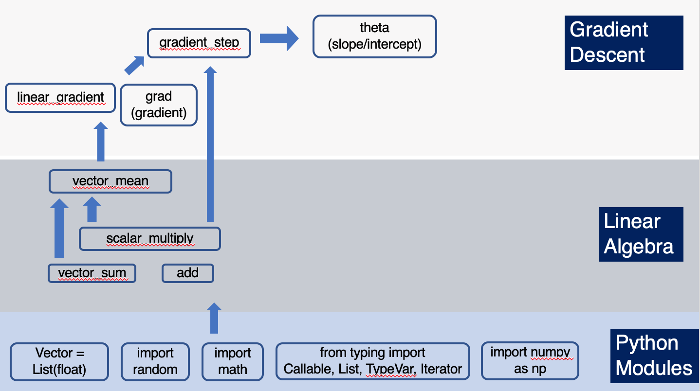
NOTE: This section builds heavily on a previous post on linear algebra. You'll want to read this post to get a feel for the functions used to construct the functions we see in this post.
from typing import TypeVar, List, Iterator
import math
import random
import matplotlib.pyplot as plt
from typing import Callable
from typing import List
import numpy as np

x = np.array([2, 4, 5])

# instead of putting y directly, we'll use the equation: 20 * x + 5, which is a direct representation of its relationship to x

# y = np.array([45, 85, 105])

# both x and y are represented in inputs
inputs = [(x, 20 * x + 5) for x in range(2, 6)]
First, we'll start with random values for the slope and intercept; we'll also establish a learning rate, which controls how much a change in the model is warranted in response to the estimated error each time the model parameters (slope and intercept) are updated.
# 1. start with a random value for slope and intercept
theta = [random.uniform(-1, 1), random.uniform(-1, 1)]

learning_rate = 0.001
Next, we'll compute the mean of the gradients, then adjust the slope/intercept in the direction of minimizing the gradient, which is based on the error.
You'll note that this for-loop has 100 iterations. The more iterations we go through, the more that errors are minimized and the more we approach a slope/intercept where the model "fits" the data better.
You can see in this list, [linear_gradient(x, y, theta) for x, y in inputs], that our linear_gradient function is applied to the known x and y values in the list of tuples, inputs, along with random values for slope/intercept (theta).
We multiply each x value with a random value for slope, then add a random value for intercept. This yields the initial prediction. Error is the gap between the initial prediction and actual y values. We minimize the squared error by using its gradient.
# start with a function that determines the gradient based on the error from a single data point
def linear_gradient(x: float, y: float, theta: Vector) -> Vector:
    slope, intercept = theta
    predicted = slope * x + intercept   # model prediction
    error = (predicted - y)             # error is (predicted - actual)
    squared_error = error ** 2          # minimize squared error
    grad = [2 * error * x, 2 * error]   # using its gradient
    return grad
The linear_gradient function along with initial parameters are then passed to vector_mean, which utilize scalar_multiply and vector_sum:
def vector_mean(vectors: List[Vector]) -> Vector:
    """Computes the element-wise average"""
    n = len(vectors)
    return scalar_multiply(1/n, vector_sum(vectors))

def scalar_multiply(c: float, v: Vector) -> Vector:
    """Multiplies every element by c"""
    return [c * v_i for v_i in v]

def vector_sum(vectors: List[Vector]) -> Vector:
    """Sum all corresponding elements (componentwise sum)"""
    # Check that vectors is not empty
    assert vectors, "no vectors provided!"
    # Check the vectors are all the same size
    num_elements = len(vectors[0])
    assert all(len(v) == num_elements for v in vectors), "different sizes!"
    # the i-th element of the result is the sum of every vector[i]
    return [sum(vector[i] for vector in vectors)
            for i in range(num_elements)]
This yields the gradient. Then, each gradient_step is determined as our function adjusts the initial random theta values (slope/intercept) in the direction that minimizes the error.
def gradient_step(v: Vector, gradient: Vector, step_size: float) -> Vector:
    """Moves `step_size` in the `gradient` direction from `v`"""
    assert len(v) == len(gradient)
    step = scalar_multiply(step_size, gradient)
    return add(v, step)

def add(v: Vector, w: Vector) -> Vector:
    """Adds corresponding elements"""
    assert len(v) == len(w), "vectors must be the same length"
    return [v_i + w_i for v_i, w_i in zip(v, w)]
All this comes together in this for-loop to print out how the slope and intercept change with each iteration (we start with 100):
for epoch in range(100):     # start with 100 <--- change this figure to try different iterations
    # compute the mean of the gradients
    grad = vector_mean([linear_gradient(x, y, theta) for x, y in inputs])
    # take a step in that direction
    theta = gradient_step(theta, grad, -learning_rate)
    print(epoch, grad, theta)

slope, intercept = theta

#assert 19.9 < slope < 20.1,  "slope should be about 20"
#assert 4.9 < intercept < 5.1, "intercept should be about 5"
print("slope", slope)
print("intercept", intercept)
Iterative Descent
At 100 iterations, the slope is 18.87 and intercept is 4.87 and the gradient is -32.48 (error for the slope) and -8.45 (error for the intercept). These numbers suggest that we need to decrease the slope and intercept from our random starting point, but our emphasis needs to be on decreasing the slope.

At 200 iterations, the slope is 19.97 and intercept is 4.86 and the gradient is -1.76 (error for the slope) and -0.48 (error for the intercept). Our errors have been reduced significantly.

At 1000 iterations, the slope is 19.97 (not much difference from 200 iterations) and intercept is 5.09 and the gradients are markedly lower at -0.004 (error for the slope) and 0.02 (error for the intercept). Here the errors may not be much different from zero and we are near our optimal point.

In summary, the normal equation and regression approaches gave us a slope of 20 and intercept of 5. With gradient descent, we approached these values with each successive iterations, 1000 iterations yielding less error than 100 or 200 iterations.
From Scratch
As mentioned above, the functions used to compute the gradients and adjust the slope/intercept build on functions we explored in this post. Here's a visual showing how the functions we used to iteratively arrive at the slope and intercept through gradient descent was built:
Take Away
Gradient descent is an optimization technique often used in machine learning and in this post, we built some intuition around how it works by applying it to a simple linear regression problem, favoring code over math (which we'll return to in a later post). Gradient Descent is useful if you are expecting computational complexity due to the number of features or training instances.
We placed gradient descent in context, in comparison to a more analytical approach, normal equation and the least squares method, both of which are non-iterative.
Furthermore, we saw how the functions used in this post can be traced back to a previous post on linear algebra, thus giving us a big picture view of how the building blocks of data science and an intuition for areas we'll need to explore at a deeper, perhaps at a more mathematical, level.
This post is part of an ongoing series where I document my progress through Data Science from Scratch by Joel Grus.
For more content on data science, machine learning, R, Python, SQL and more, find me on Twitter.


